The catalogue has 5,000 product photographs, and the unit retrains a small classifier every month as new products arrive. The question is not "which GPU is best" but "which accelerator fits this workload, this deadline and this budget". The one big idea for this session: choosing an accelerator is a measurement — of memory, time, throughput and cost — not a badge.
The lab trains the same 298,858-parameter CNN on the same 6,000 images on this MacBook, a free Kaggle T4 and the faculty RTX Pro 6000. Only the device changes. The comparison table is the deliverable, and the capstone brief carries the habit into the final project.
Lesson
What training needs
A training run needs data, a model, a loss, an optimizer and a number of epochs. The data and the model decide how much memory is required; the optimizer and the batch size decide how much more. The device decides how fast the arithmetic runs and how much of it can run at once.
Two numbers describe a run: time to finish and peak memory. A third describes how well the device was used: utilization. A run that finishes in two minutes at 15% utilization is not a fast device; it is a small job on a large one.
The roofline in one page
A roofline compares a workload's arithmetic intensity — operations per byte moved — with the device's memory bandwidth and peak compute. Low intensity means memory-bound: the device waits on data. High intensity means compute-bound: the device waits on arithmetic.
Training a small CNN on 28×28 images is mostly compute-bound but sensitive to batch size and data loading; inference at batch 1 is often memory-bound. The same device can look fast on one and slow on the other. That is why the lab fixes the model, data and epochs, and varies only the device.
Time, memory and warm-up
The lab reports seconds per epoch and the total. The first epoch on Apple MPS includes graph compilation, so it is slower than the rest; the comparison reports the mean seconds per epoch, quotes the first epoch separately and gives the total, because a single total would hide the warm-up.
Peak memory matters because it decides what fits. The small CNN peaks at 1.13 GB on the Mac's MPS path and 0.16–0.19 GB on the two CUDA cards — comfortably inside a 16 GB T4 and far inside the 96 GB RTX card. The gap is mostly the framework: MPS reports driver-allocated memory, CUDA reports the peak of allocated tensors. A larger model, a bigger batch or a longer sequence moves the requirement; the device must fit the workload, not the reverse.
Cost
The cost of a run is hourly price × hours used, plus data transfer and the cost of idle time. A free T4 is free within its weekly quota; the faculty card is free to the student but not free to the institution; a rented RTX Pro 6000 is about $1.69/hour on RunPod's secure cloud, so a 10-minute run is about $0.28. The notional line in the lab's table keeps the comparison honest without pretending the faculty card was rented.
For a monthly retraining job that finishes in minutes, the cheapest adequate device usually wins. Renting a 96 GB card for a 1.1 GB job buys capacity the job cannot use.
Choosing for the unit
A workable decision rule:
Fit memory first. Does the model, batch and data fit? If not, the device is out.
Meet the deadline. Is the run short enough for the retraining window? If not, move up.
Price the run. Compare hourly cost × time, not hourly cost alone.
Check availability. A free device you cannot book is not available; a rented card you forget to stop is not cheap.
The lab's three rows are the evidence for the rule. The research question asks the student to apply it to captions and image classification, with a fallback.
Transfer learning
Transfer learning reuses a model trained on one task as the starting point for another. It is why a small labelled media dataset can still produce a useful classifier, and why the choice of accelerator is often about fine-tuning a backbone rather than training from scratch. The lab's CNN is deliberately small and from scratch; the capstone may use a pretrained backbone, which changes the memory and time budget.
The capstone
The capstone keeps the same unit and the same catalogue, and it is where the course's threads meet. The common brief: design and prototype the next phase of the unit's catalogue — add AI tagging to the 5,000-asset library, with a governance rule, inside a fixed monthly budget. You choose the tagging method — managed inference (S8), the fine-tuned Qwen3.5-4B (S9) or an image classifier (S10) — and justify it against the fact sheet.
The substrate is not free choice: it is the stack the course built. Private R2 holds the canonical catalogue and the tags, reached only through the Worker's binding. Public R2 serves the 400 px thumbnails through media.<root>; it is a different bucket because an R2 custom domain exposes every key in the bucket it is attached to, and the catalogue must never be public. The Nextcloud/RAID1 NAS holds the 5,000 originals as the local working library and mirrors them to R2 — it is the origin and the backup, not the catalogue database. The S4 Worker is the catalogue API and the write gate. OpenRouter is the managed inference path, and its endpoint policy is enforced on every request. Each piece has one job because each piece fails differently: losing the NAS loses the originals, losing R2 loses the catalogue, and a Worker without a gate writes whatever it is sent.
The starter pack at course/samples/capstone/ is the beginning, not the answer. It ships a seeded generator for the 5,000 synthetic assets and their manifest, a tagging pipeline with a preflight, checkpointed batches of 100 and a resumable failure log, the S5 Compose stack for the NAS, the S4 Worker extended with a tag-ingest route, the governance rule, a budget sheet with its reconciliation, and a verifier. COMMANDS.md lists every command in order with an explanation; read it before you run anything.
Governance is enforced, not asserted. The rule is the S8 six-part rule extended with the tag schema and the 10% review sample. Before any request, the pipeline checks the dated endpoint snapshot for an endpoint that actually meets the rule — zero data retention, no data collection, no fallbacks — and refuses to start if none does. Every record is validated locally, then validated again by the Worker, which writes nothing if one record in a batch fails. The evidence is a refused request and an accepted governed write: a 4xx from a pinned non-ZDR endpoint, then a 200 from a qualifying one. A rule that is only described in a report is not a control.
The budget is a shape, not a wish. The monthly spine is $80: storage $25, compute and CDN $25, egress $15, inference $5 and a $10 buffer. The inference line is fixed at $5/month and measured from one 40-item monthly batch projected to the monthly run-rate; the one-off backfill is capped at the $10 OpenRouter credit from S8. Cloud resources run in a bounded 72-hour window and are torn down, so the compute and storage lines are window costs — about $2.56, not a month of Droplet — while R2, Workers and egress stay inside their free tiers. You report actuals and explain every delta; editing the spine to make a number fit is the failure mode the reconciliation exists to catch.
The proposal is a 1,000-word brief with the four components — R2's private and public buckets, the NAS, the Worker and OpenRouter — and their data flows, a three-row risk-register seed, the budget arithmetic, a feasibility calendar and your method choice. It is due one week after this session. The implementation tags all 5,000 assets, and the pass mark is at least 99% schema-valid; classifier users also report holdout accuracy on the generator's 200-asset labelled set, while captioning users rely on the 10% review. The implementation and the 2,500-word report with a 10-minute presentation follow outside the ten weeks. The rubric is in the assessment scheme; the full brief, the ten-item evidence bundle and the fallback chain are in the starter pack's README.md.
If a component is unavailable, the fallback chain keeps the evidence shape: workers.dev plus r2.dev without a zone, the instructor demo bucket plus wrangler dev --local without an R2 subscription, local Compose for the NAS without a Droplet, a free-tier or instructor OpenRouter key without a card, and MPS or CPU without a GPU. Label every substitution in your note. A fallback that changes what you can prove is a defect.
Check yourself
Why is seconds per epoch a better comparison than total seconds when the first epoch is a warm-up?
A model peaks at 1.1 GB and trains in 18 seconds. Which device fits, and why is the 96 GB card a poor default?
Your monthly retraining window is one hour. The T4 takes 45 minutes and the rented RTX takes 5; what else do you need to know before choosing?
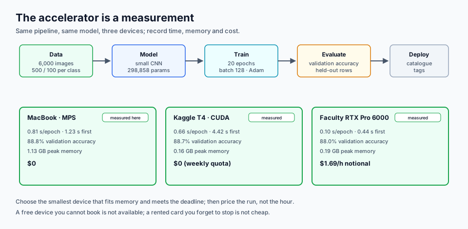
Figure 10.1 — The accelerator is a measurement: the same pipeline, the same model, three devices, and a table that records what each one cost in time and memory.
Reading the figure. The top row is the pipeline every device runs: the bundled 6,000-image dataset, the 298,858-parameter CNN, 20 epochs of training, validation accuracy, and the catalogue as the deployment target. The three cards below are the devices, and all three are measured. The footer states the rule: choose the smallest device that fits memory and meets the deadline, then price the run.
Configuration
Device
Epochs
Seconds/epoch
Validation accuracy
Peak memory
Notional cost
MacBook (MPS)
Apple M1 Max
20
0.81 (1.23 first)
0.888
1.13 GB
$0
Kaggle T4
CUDA, 16 GB
20
0.66 (4.42 first)
0.887
0.16 GB
$0
Faculty RTX Pro 6000
CUDA, 96 GB
20
0.10 (0.44 first)
0.880
0.19 GB
$1.69/h notional
All three rows are the shipping notebook's runs: the Mac on the reference MacBook (Python 3.14, torch 2.10.0, numpy 2.5.4), the T4 in a Kaggle GPU session (Tesla T4, torch 2.11.0+cu130), and the RTX card on the faculty host (torch 2.12.1+cu130, driver 610.57.04). The Mac row is one 20-epoch run; repeated Mac runs moved the mean seconds per epoch and the total by a few percent while accuracy and peak memory stayed put. The table is the same information as the figure.
Why the GPU number moves between runs. With the same seed, data and hyperparameters, repeated runs on a GPU validated a point or two apart — six RTX runs spread 0.875–0.893 — while seconds per epoch and peak memory stayed put. cuDNN picks kernels per run and does not promise bitwise-identical arithmetic, so a GPU row is one measurement, not a constant. Record what your run printed, note the spread if you run twice, and compare seconds per epoch rather than chasing the last digit of accuracy.
Prerequisite: A phone-verified Kaggle account for the T4 run and the faculty RTX card (or the RunPod fallback); the kit's S10 dependency group or the light install. Set it up in Session 0: Accounts, Tools.
Lab — three-configuration training comparison and capstone brief
Time: 120 minutes — 15 setup, 70 for the three device runs (the Mac is pre-lab), 20 for the table and cost, 15 for evidence and the capstone outline. The Mac run is the pre-lab self-study task; the in-class block runs the T4 and the RTX card, then merges.
Prerequisite: S9; Python 3.14; the bundled dataset at data/fashion_subset.npz (6,000 Fashion-MNIST images, MIT, 2.6 MB, no download). The provenance and licence are in data/README.md.
You need to know: the same model and data on different accelerators isolates the device; seconds per epoch, peak memory, utilization and cost are the comparison; the first epoch may include a warm-up.
Safe-data acknowledgement: I have read the lab safe-data policy. I will use only the course-supplied synthetic media and will not upload real personal media to any cloud service.
Task
Train the same 298,858-parameter CNN on this MacBook, a free Kaggle T4 and the faculty RTX Pro 6000, merge the three runs into one comparison table, and recommend an accelerator for the unit's monthly retraining — then outline the capstone proposal.
Steps
1. Pre-lab: run the Mac
Before class, open notebook.ipynb and run the cells with S10_LABEL=mps (the default). The notebook takes its settings from environment variables, so in Jupyter put %env S10_LABEL=mps in a cell above the settings cell; from a shell, start Jupyter with S10_LABEL=mps jupyter lab. The full run is about 20 seconds on MPS and writes results/mps.json; the merge cell then writes results/comparison.csv. Bring the JSON to class.
# Optional CLI check on the Mac
python3 -c "import torch; print(torch.__version__, torch.backends.mps.is_available())"
2. In class: run the Kaggle T4
Console: create a private Kaggle notebook (Settings → Accelerator → GPU T4 ×2; the notebook uses one), and upload data/fashion_subset.npz to the working directory.
Add %env S10_LABEL=t4 as the first cell — Kaggle gives you no shell to export a variable into, so the magic sets it for the kernel — then run the cells and download results/t4.json. The settings cell asserts it sees CUDA, so a T4 that failed to attach stops the run instead of quietly writing a CPU row. Record the GPU name and the utilization from nvidia-smi while the run is active:
Copy the dataset and notebook to the faculty machine's course workspace (or use the shared folder). Put %env S10_LABEL=rtx and %env S10_HOURLY_COST=1.69 in a cell above the settings cell — 1.69 is the notional RunPod secure price; the faculty card itself costs the student nothing. Run the cells, capture the utilization screenshot, and copy results/rtx.json back to the Mac.
If you use RunPod instead: book a 45–60 minute slot on the instructor-owned account, use a PyTorch image, upload the 2.6 MB dataset and the notebook, set auto-stop to 30 minutes idle, and terminate the pod and its network volume at the end. The 10-minute run costs about $0.28 at $1.69/hour.
4. Merge and price the comparison
Put all three JSONs in results/ and run the merge cell. It writes results/comparison.csv. Fill the cost column: Mac $0; T4 $0 within the weekly quota; RTX $0 to the student plus the notional RunPod line; RunPod actual = hourly price × hours used, plus any volume charge.
Read the table and answer:
Which device was fastest per epoch, and how much of the difference is the first-epoch warm-up?
What does the peak memory mean for a 16 GB T4 versus a 96 GB card?
Which device would you choose for the unit's monthly retraining, and what would change your mind?
5. Write the evidence note
Write 150–250 words: the comparison, the cost line, the utilization observation and the recommendation. Attach comparison.csv, the three JSONs and the utilization screenshot. A screenshot of a bill is not a utilization screenshot.
6. Outline the capstone proposal
In the last 15 minutes, draft the outline for the revised capstone, which starts in earnest after this session. The common brief is to add AI tagging to the 5,000-asset library, with a governance rule, inside a fixed monthly budget, on the course stack. The starter pack is course/samples/capstone/; read its README.md and COMMANDS.md before you start, and do not begin the implementation until the proposal names every component.
Sketch:
the problem and scope in one paragraph;
an architecture diagram with four components and their data flows: R2 with its private catalogue/tags bucket and its public thumbnail bucket labelled separately, the Nextcloud/RAID NAS as origin and backup, the Worker as the API and write gate, and the inference path — managed OpenRouter, the fine-tuned Qwen3.5-4B, or the S10 classifier;
the governance rule: the S8 six-part rule plus the tag schema, where the dated endpoint snapshot is checked before sending, and where the Worker refuses a non-compliant record;
the risk-register seed: three rows from S7/S8, each with its control;
the budget arithmetic: the $80 spine, the fixed $5 inference line, the $10 one-off backfill cap, and what the bounded 72-hour window does to the compute and storage lines;
the feasibility argument, including the accelerator choice from this lab and the 5,000-asset run in batches of 100;
the method choice and why it beats the other two for this catalogue.
The full 1,000-word proposal is due one week after this session; this outline is the in-class start, and the one-hour self-study block finishes it. The implementation must tag all 5,000 assets with at least 99% schema-valid records and prove the gate with a refusal and an accepted governed write. The report is 2,500 words with a 10-minute presentation and 5 minutes of questions.
Evidence bundle
results/comparison.csv and the three result JSONs.
A GPU utilization screenshot from the T4 and the RTX card (or the RunPod pod).
The 150–250 word what this proves note with the recommendation.
The capstone proposal outline.
A teardown log: Kaggle session stopped, faculty kernel stopped, RunPod pod and network volume terminated, budget checked.
The bundle is scored 3/2/1/0.
Failure and recovery
The deliberate failure is mislabelling a device: run the notebook on the Mac with S10_LABEL=t4 and watch the assertion refuse it. The table must record what actually ran; a borrowed row is labelled borrowed and a measured row is labelled measured. If the RTX card is unavailable, the T4 becomes the third configuration and the note says so. If both GPUs are unavailable, use the instructor's precomputed rtx.json, label it borrowed, and still run the Mac row. Never fill a GPU row with an estimate and call it measured.
Cost ceiling
$0 on the Mac, the free T4 and the faculty card. A RunPod fallback is under $3.40 at $1.69/hour for two hours; the lab run itself is about $0.28. The dataset is 2.6 MB, so transfer is negligible. There is no persistent storage.
Teardown
Mac: stop the kernel; copy results/; delete the run folder.
Kaggle: stop the session after downloading the JSON and screenshot.
Faculty RTX: stop the kernel and remove the outputs from the shared workspace.
RunPod: terminate the pod and its network volume; confirm the billing page shows no running instance. An auto-stop is not a teardown.
Fallback
T4 as the third configuration if the RTX card is unavailable; the instructor's precomputed RTX JSON if neither GPU is available, labelled borrowed. The Mac path always works. The evidence shape does not change.
Notebook
Open the lab notebook; run it once per device with S10_LABEL set to mps, t4 or rtx. It writes one JSON per run, then merges comparison.csv.
Downloads for this session
Each document name opens a rendered view you can read in the browser. The download link beside it gives you the raw Markdown working file: the copy you edit, run and submit. The page above and the lab steps carry the teaching.
The runnable notebook that produces the lab's numbers.
Research question
How should the unit choose between a workstation GPU, a free T4 and the faculty RTX Pro 6000 for a given training task?
Submit an 800–1,200 word answer with 5–8 sources at the next session. The rubric and the exemplar guidance show the expected shape.
References — Session 10
Krizhevsky, A., Sutskever, I., & Hinton, G. E. (2012). ImageNet classification with deep convolutional neural networks. Advances in Neural Information Processing Systems 25; reprinted in Communications of the ACM, 60(6), 84–90 (2017). https://doi.org/10.1145/3065386
The result that made GPU training the default for image media, and the reason the course spends a session on accelerators. Energy and cost per useful media model are rarely reported alongside accuracy. The architecture diagram is widely reproduced; redraw it.
He, K., Zhang, X., Ren, S., & Sun, J. (2016). Deep residual learning for image recognition. 2016 IEEE Conference on Computer Vision and Pattern Recognition (CVPR), 770–778. https://doi.org/10.1109/CVPR.2016.90
Residual connections make deep networks trainable and give students the transfer-learning backbone the capstone may use. Efficient fine-tuning of residual backbones on small media datasets is still an empirical craft. The residual-block figure is a redraw candidate.
Jouppi, N. P., Young, C., Patil, N., et al. (2017). In-datacenter performance analysis of a tensor processing unit. Proceedings of ISCA '17, 1–12. https://doi.org/10.1145/3079856.3080246
Introduces the roofline reasoning students use to explain why a GPU is memory-bound or compute-bound. Roofline models for workstation cards in media pipelines are less studied than datacenter accelerators. The roofline chart can be rebuilt from the paper's method.
Dosovitskiy, A., Beyer, L., Kolesnikov, A., et al. (2021). An image is worth 16x16 words: Transformers for image recognition at scale. International Conference on Learning Representations (ICLR). https://arxiv.org/abs/2010.11929
Shows the data/compute trade-off that decides whether a transformer or a CNN is the right choice for a media task. ViT efficiency on small, domain-specific media datasets remains an active question. The patch diagram can be redrawn.
Teaching note. Narrate Krizhevsky et al. (2012) for 5–8 minutes, assign the abstract of Jouppi et al. (2017) as reading, and close by restating the open problem as the weekly question. Figures are third-party; redraw by default.
PLO — Session 10: Image ML on a GPU + capstone
CLO: By the end of this session, the student can train the same image classifier on three accelerators, compare time, memory, utilization and cost, recommend a device for a monthly retraining job, and frame the capstone proposal on the revised R2/NAS/Worker/OpenRouter stack.
PLO
Role
Research answer
Lab evidence
Points
Evidence
Rubric
PLO1
primary
4
3
7
An 800–1,200-word accelerator-choice analysis with 5–8 sources; the comparison CSV, three JSONs, utilization screenshot, cost line, recommendation and capstone proposal outline (five components and data flows, governance gate, $80/$5/$10 arithmetic, method choice)
Research 4/3/2/1; Lab 3/2/1/0
PLO2
secondary
0
0
0
Lecture context only; not scored
—
PLO3
secondary
0
0
0
Lecture context only; not scored
—
Total
4
3
7
Total: 7 points
Four-level descriptors
Research (4/3/2/1). 4 = a decision rule (memory fit, deadline, cost, availability) applied to captions and image classification with the measured table, a fallback and a counterargument about renting versus free quota. 3 = a sound comparison with a recommendation and most of the rule. 2 = lists device specifications without choosing or using measurements. 1 = a summary with fewer than five sources. 0 = nothing submitted or misconduct.
Lab (3/2/1/0). 3 = three configurations recorded (or the fallback labelled honestly), the comparison table and cost are correct, the utilization evidence is present, the recommendation uses the numbers, and teardown is complete. 2 = mostly complete, one row or check thin. 1 = one or two rows, an estimated row presented as measured, or incomplete teardown. 0 = nothing submitted, unsafe data, or no teardown.
The full course arithmetic is in production/baseline.md; this file is the weekly instance.